In the early 1980's, C.F. Aquino from Ford published a SAE document on "wall wetting compensation", and how it was implemented in the Ford CFI setup. The concept of wall-wetting is very simple: for every squirt of the fuel injector, the majority of the fuel makes it into the cylinder, but some of the fuel from the squirt collects on the wall of the intake manifold and intake valve. In simplistic terms, a certain percentage of fuel (call this (1-X)) gets into the cylinder, the remainder sticks to the walls (call this X), hence the term 'wall wetting'.
The fuel that sticks to the walls eventually evaporates back into the airstream and is drawn into the cylinder. This is a time variable, call it Tau (= τ is the Greek letter frequently used in scientific literature to represent time), which is the amount of time it takes to get the fuel clinging to the wall back into the cylinder.
That's all there is to it, for every squirt a certain percentage sticks to the walls, and at the same time the fuel on the walls is dissipating back into the airstream. Think of it like taking a paintbrush filled with paint thinner and brushing it on a wall, some of it sticks to the wall on every stroke, but eventually it will evaporate away. Glob on a thicker coat and it takes longer to evaporate, or put on many fast strokes. If you stroke more often then the acetone will start to build up, since you are applying a new coat before the old one dissipates. And if the air temperature is warmer it will evaporate faster than if the air is cold.
X-Tau is the same thing, for every injection part of the squirt clings to the manifold, valve, etc. It will eventually evaporate, but the stuff that clings to the wall is not getting into the cylinder immediately. For steady-state conditions this is OK because fuel is evaporating and being re-deposited at the same time to reach an equilibrium. But during a throttle transition more fuel is required outside of this equilibrium due to the increase in air flow (per unit time). But if a percentage of the fuel clings to the wall then in these situations more fuel needs to be added (longer pulse width) to compensate. Of course, then a bit later, when the fuel starts evaporating, the situation changes and there is now too much fuel, so the pulse width is backed off. This gives the characteristic fast rich/lean jump - but this deviation maintains the tightest excursion range for AFR.
It is interesting in that the latest ULEV (Ultra-Low Emission Vehicles) control strategies use X-Tau for both transient enrichment and warmup enrichment, in two separate loops ( a slow one and a fast one). These vehicles maintain a target AFR right from cranking (and all operating conditions at all times) and it cannot deviate outside of a tight tolerance. And the Tau time constants for warmup have evaporation values in the "many seconds" range, it takes a while for cold fuel to vaporize off of a cold valve or manifold. As the temperatures increase so does the evaporation rate, so Tau gets smaller. Also, the percentage of fuel that actually sticks when squirted (the X) changes, so there are X defining tables as well as a function of coolant temp.
Note that if the injection pulse width is the same, and if it arrives with a fixed time interval (i.e. same RPM) then a equilibrium is reached where the amount of fuel sticking to the walls is in equilibrium with the wall film dissipating back into the airstream. However, a change in pulse width or a change in the time between injections upset this equilibrium, requiring an "adjustment" in the delivered fuel if one wants to compensate, hence the term "transient fuel compensation".
The method is known as "X-Tau" compensation, where you specify:
Both can be a function of RPM/MAP, coolant temp, etc. From many of the SAE docs the broad conclusion is that the X value is pretty much the same but the Tau is a function of several parameters - but this is a pretty generic assessment.
X-Tau transient enrichment compensation is in the MegaSquirt-II™ V2.6+ code. Here is the header from a simulation file:
Code:

/**************************************************************************
**
** X,Tau Transient Enrichment Section:
**
**   fi = [ mi - (Mi / (tau / dltau)) ] / (1 - X)
**
**   Mi+1 = Mi + X * fi - (Mi / (tau / dltau))
**
**  where,
**       fi = total fuel injected
**
**       mi = total fuel going directly into combustion chamber (want this
**           to be the calculated fuel)
**
**       Mi = net fuel entering/leaving port wall puddling
**
**       dltau = time (secx100) between tach pulses = dtpred
**
**       X = fraction of fuel injected which goes into port wall puddling
**       tau = puddle fuel dissipation time constant (secx100) as function
**           of map, rpm, coolant temp and air temp.
**
**      XTfcor = % correction to calculated fuel to ensure the calculated
**           amount gets into the comb chamber.
**
**************************************************************************/
Here is a plot simulating an acceleration and deceleration event (each back to original PW):
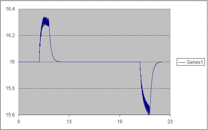
Note that the injected pulse width is increased then ramps back down (in a smooth fashion) for the acceleration (the same for decel, but in the other direction). You can see that there are little oscillations in the fuel waveform where it is over/under compensating, this is an artifact from the discrete nature of the algorithm (note that this variation is in the microsecond range).
Here is an image from a 1984 Toyota patent (number 4,388,906) which shows the improvement in AFR with the X-Tau method compared to no compensation:
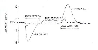
Note that this is air-fuel ratio, and you can see the lean "tip-in" during acceleration being corrected by the adjustment in fuel computed by the X-Tau method.
The X-Tau table implemented in MegaSquirt-II™ code (V2.8+) has six tables.
The Tau table entries represent the dissipation time of the fuel on the wall. As rpm goes up, the fuel evaporates faster (table entries become smaller); as map goes up the fuel takes longer to dissipate. That is why you need an initial enrichment, but it is less at high rpm.
This algorithm should help users with acceleration enrichment issues, particularly lean tip-in. In fact, this method should in theory be the main acceleration enrichment, but we will have to see how it works in practice. Also note that improper selection of X and Tau can lead to a run-away in injected fuel. For example, an extreme case (and totally incorrect) is where someone puts in, say 99% for X (i.e. pretty much all of the fuel sticks to the walls). In this case the computed pulse width correction will jack the fuel up so much that the injector will most likely be on all of the time, and this is not good for a running engine. So, care will need to be exercised when coming up with X and Tau.
It is important that people do not choose extreme values for the X part of X-Tau. For those that just want the bottom line, if you keep you X below 48%, you shouldn't have to worry about oscillation and this is a very large puddling factor.
The table below shows the range your Tau values should be greater than. The data was obtained from a simulation of the X-Tau loop in the MegaSquirt-II code. So if people are going to try to push the edge of the table, they should go through all the map/VE entries on the stim and make sure it never gets into oscillation. Fortunately it is more likely to oscillate at low rpm than high rpm. To avoid oscillation tau must be greater than (or equal to) the table entry to avoid oscillation:
| Oscillation Table: tau must be >= table entry to avoid oscillation | |||||||||||||||
| RPM | 50 | 500 | 1000 | 1500 | 2000 | 2500 | 3000 | 3500 | 4000 | 4500 | 5000 | 5500 | 6000 | 6500 | |
| X | 90 | 1.80 | 0.18 | 0.09 | 0.06 | 0.05 | 0.04 | 0.03 | 0.03 | 0.03 | 0.02 | 0.02 | 0.02 | 0.02 | 0.02 |
| 80 | 0.90 | 0.09 | 0.05 | 0.03 | 0.03 | 0.02 | 0.02 | 0.02 | 0.02 | 0.01 | 0.01 | 0.01 | 0.01 | 0.01 | |
| 70 | 0.60 | 0.06 | 0.03 | 0.02 | 0.02 | 0.02 | 0.01 | 0.01 | 0.01 | 0.01 | 0.01 | 0.01 | 0.01 | 0.01 | |
| 60 | 0.60 | 0.06 | 0.03 | 0.02 | 0.02 | 0.02 | 0.01 | 0.01 | 0.01 | 0.01 | 0.01 | 0.01 | 0.01 | 0.01 | |
| 50 | 0.60 | 0.06 | 0.03 | 0.02 | 0.02 | 0.02 | 0.01 | 0.01 | 0.01 | 0.01 | 0.01 | 0.01 | 0.01 | 0.01 | |
| 48 | 0.01 | 0.01 | 0.01 | 0.01 | 0.01 | 0.01 | 0.01 | 0.01 | 0.01 | 0.01 | 0.01 | 0.01 | 0.01 | 0.01 | |
Note: In code versions 2.850+, Tau = 0 is allowed so people can exclude certain regions from getting X-Tau fueling adjustments. You still need to keep Tau > the table values, but you can also set it to 0. (For example if the table says keep it > 3, then do not set to 1 or 2, but you can set Tau to 0.) What will then happen is the code will set the actual Tau to 1 (otherwise it would be dividing by 0), but will ignore the X-Tau fuel correction. The reason for this is that this way the X-Tau loop remains in operation so that when you get back into a region where you want to use it, everything will be instantly ready in the loop, and the correction will be turned back on.
Note that the X-Tau implementation in the code has been somewhat simplified in recent code versions. The original MS-II implementation of X-Tau was a bit complicated with a lot of inputs which was one of the major impediments for successful results.
Also, this first implementation existed with the asynchronous MAP sampling scheme, where the MAP signal was sampled in a time-based manner, and not relative to engine cycle. The result was significant MAP deviations that were not indicative of mass air flow. Anyone with an o-scope can see this - run the vehicle at idle and hook the scope to the output of the MAP sensor, you will see a sine-wave like modulation on the DC signal - we want the DC signal, not the cycle-to-cycle variations. Imagine if the sampling was not synchronized to the phase of this wave - this is what we used to have. With the MAP reading bouncing around, the "knee-yank" solution was to jack up the low-pass lag filter for MAP - but this also killed x-tau response for fast transients. With the synchronous (crank-position based) MAP sampling and the simplified X-Tau inputs, the general transient-enrichment method has really been improved. (Note to those testing X-Tau - go to the lag filter and reduce the lag value, the default still has a bit of averaging).
There are a number of user-configurable settings for X-Tau:
If X-Tau is enabled under 'Settings/General/X-Tau Usage', then you'll find:
As a tuning tip, people should start with low X and low Tau (default values until you get something better). You should then see if the X-Tau helps. Start by adjusting the X factor. If that doesn't help, try increasing the Tau time table entries in the areas where you are having troubles with lean spots (engine coughs on accel).
The Tau time table is deliberately conservative, so in most cases it will require increasing, by perhaps 50% to 100%.
You may need to try adjusting the lag filter values for the MAP sensor for less filtering. The X-Tau mode needs to see the rapid rate-of-change of MAP and the lag filters can reduce this if set too low. Generally you do not want to set it to less than 50%, and may need to set it to 70% to 80%.
T As you dial-in the X-Tau parameters, the engine will likely become overly rich due to both normal and X-Tau enrichments being applied. You can try reducing the existing TPSdot or MAPdot based accel/decel enrichments, which do NOT go away when you specify the X-tau option and increasing the X-tau variables. (Note that you may have to increase the cold accel multiplier as you do this.)
The position of the MAP sensor tap point as it pertains to X-Tau use was addressed in the Overgton/Hires SAE paper on transient enrichment. In the paper they modeled the mass airflow and the effect of the pulsation in each runner due to the position of the piston, valve opening phase, and the volume of the manifold, and compared this to actual measured data (with excellent results). The short version of the conclusion was that MAP sensor placement was not a critical factor in transient compensation.
In regards to MAP sensor signal ripple at low RPMs, the way that MegaSquirt® operates factors a lot of this out by sampling at the same point (to first order). With the main loop running at a rate of a few milliseconds and the ADC channel acquisition occurring at roughly the same rate, there are many, many runs through all of the calculations, but the one that is actually used for PW is the one right after the last injection pulse. Since the injection pulse timing is tied to crank position via. the tach pulse, the pulse width that is used has a strong synchronization to the crank. It is not perfect, and issues like valve overlap and the like will alter this but its also not a totally random event.
A graph is worth a thousand words:
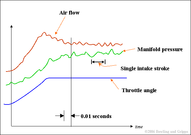
The throttle angle is shown on the bottom trace, it ramps from a closed position to a more open position then stops moving and stays in the same position. The middle trace is the reading from a MAP sensor taken from the manifold plenum. The top trace is the instantaneous measured mass airflow. A few things to see in the plot:
1) Note the amplitude of the ripples in the MAP sensor, and the overall amplitude of the MAP signal trend. The trend dominates over the individual ripples (for this case). The ripple magnitude depends on factors like RPM, sensor response, manifold+runner volume, etc.
2) Note the time scale of 10 milliseconds, and note the length of time of a single intake stroke (although RPM dependent). This may help answer the question of phase delay of MAP signal due to port placement and/or length of vacuum tubing. For MAP delay due to the low pass filtering caused by the RC input filter, the R is 1K Ω and the C is 0.22µF, giving a time constant of 220 microseconds (at 63%) - not a real factor here in comparison.
3) The extremely interesting thing here is the air flow. Notice the point where the throttle stops moving, the air flow rate reaches a maximum and actually starts slowing down to an equilibrium value. This is known as air charging, where the capacitive effects of the manifold/runner volume and the increasing air density peak when the throttle is moving, then settles back down. Note that the trend of the MAP reading does not indicate this - the MAP pretty much follows the throttle (or TPS) angle.
The Aquino paper really addresses the air charging effect. In fact, if there was no such thing as air charging then the X-Tau algorithm would really be simple, just (1-X)*MeteredFuel + (1/Tau)*MassOfFilm. Taking the air charging into account complicates the calculation a bit. This can be seen in the actual AFR readings during a transient with X-Tau, with the characteristic rich-then-lean humps, corresponding the rate-of-change of the mass air introduction into the manifold.
Here is a video of Dr. Jim Cowart's* presentation on X-Tau:
*(Dr. Jim Cowart is a professor at the US Naval Academy. His direct assistance on the X-Tau method has been extremely productive. For those not familiar with him, he worked for Ford calibration department for 10 years before moving on to obtain his doctorate from MIT in engine controls (dissertation was in evaluating wall wetting phenomenon). He reviewed our X-Tau implementation (first, realize someone of his caliber and stature taking the time to look over a DIY project like MegaSquirt®, this is pretty significant). His feedback we directly implemented in the current code and the user inputs.)
It should be noted that Dr. Cowart is using MegaSquirt® on one of his upcoming research projects. He also heads up the FSAE team for US Naval Academy, and they are using MicroSquirt® for their controller. Also, for those who like to learn from the best, go to the Society of Automotive Engineers (SAE) website at www.sae.org, and search for the name "Cowart". Purchase some of the papers (along with the Aquino paper 810494) if you want to really understand X-Tau, among other things. The best ones are the 2007-01-0473 and the 2002-01-2753. These papers are a little "heady" so take your time and re-read them over again (and ask questions on the support forums) - the information within these documents are invaluable!